


We have mentioned that computation of aeroacoustic sound sources is
difficult. This is primarily due to the fact that in order to compute the
correct characteristics of a sound source, one needs information on the
instantaneous turbulent flow field as a function of time and space. As
turbulence itself is not analytically tractable, one way-out is to use
numerical computation with help of turbulence models. To compute the sound
source from the Lighthill equation one needs multi-point statistics
such as space-time correlations. Most computational methods for turbulent
flows, such as the widely-used  model or even the more advanced
Reynolds stress models, produce only one-point statistics. As a result not
much progress has been made with the computation of aeroacoustical sources
and the associated sound field.
model or even the more advanced
Reynolds stress models, produce only one-point statistics. As a result not
much progress has been made with the computation of aeroacoustical sources
and the associated sound field.
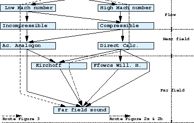 |
Nowadays, more advanced computational techniques, like Direct Numerical Simulation (DNS) and Large Eddy Simulation (LES), are available. In these techniques the Navier-Stokes are solved directly. Their main advantage is that they provide a space and time resolved flow field, from which the sound source can be directly computed. However, even in this case the computation of the sound field is far from straightforward. Figure 1 shows several computational strategies that can be adopted. The first step is in all cases to obtain the flow field as accurate as possible by means by the aforementioned DNS (low Reynolds number) or LES (high Reynolds number) methods.4 Next, depending on the Mach number of the flow one can choose for a compressible or incompressible approach.
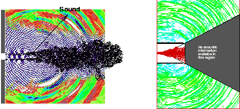 |
A compressible flow calculation is the most direct way of computing the sound source because the coupling between flow and acoustics is implicitly described by the equations. An example of our own computations with the fully compressible method is shown in figure 2 for the case of a jet flow with a Mach number of 0.6 and a Reynolds number of 3,000 (both numbers are based on jet nozzle velocity).
In figure 2(left) the turbulence flow field is illustrated by its vorticity pattern indicated by the black contour lines. The propagating sound wave is visualized by the dillatation of the velocity field, which is local rate of change of volume and which is indicated by colored contours. It is clear that the sound waves originate from the area where the shear layer of the initial jet breaks up in a chaotic vorticity pattern. However, the results shown in figure 2(left) gives us only the pattern of the near-field sound. To find the sound pattern in the far field, a full DNS computation would require too much computer resources. However, in the far field there are no sound sources and given that pressure perturbations are small, we can approximate the compressible Navier-Stokes equations by the wave equation for these pressure perturbations. The pressure perturbations are introduced on the boundaries of the computational domain, which is similar to the Kirchoff surface method used in classical field theory. The results obtained with this method are shown in figure 2(right). The sound field in the gray area in figure 2 (right) is not predictable with the Kirchoff method, because the velocity needs to be zero on the boundary where the pressure information is fed into the wave equation. This is only the case on the horizontal boundaries but not on the vertical boundary of figure 2(right).
The computational strategy, which we have followed for this case is
indicated in figure 1 by the dashed-dotted line. This
computational strategy is only suitable for high speed or high
Mach number flows, while as mentioned before, we would like to consider
low speed or low Mach number flows in the present proposal.
Therefore, we have to follow another route as shown in figure 1
by the dashed line. The reason is that for low-speed flows the pressure
fluctuations connected to sound become almost negligible with respect to
the pressure fluctuations connected directly to the velocity fluctuations.
This would require extremely accurate numerical schemes. Moreover, in this
case also large computational times are needed because the timestep is
severely limited by the acoustical wave speed. Therefore, we compute for
the low Mach number case the flow field by completely neglecting the effect
of acoustics, which in fluid mechanics is known as an incompressible flow.
The advantage of this approach is that very fast, reliable and efficient
numerical methods are available. To compute or better to reconstruct the
sound field we must then make use of a so-called acoustic analogon, like
the non-linear source term in the aforementioned Lighthill equation. The
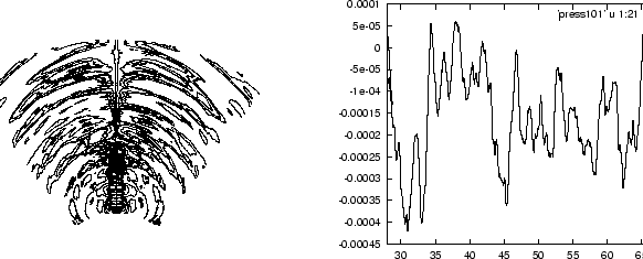
result of such a reconstruction is shown in figure 3. It should
be mentioned that in this computation additional simplifications have been
made. For instance the non-linear source term in the Lighthill equation
contains the density  . This is the total density, which includes the
acoustic component, and thus it will have spatial and temporal variations.
Therefore, to solve the equation we have linearized (as is done
in the second footnote on page 4) the source term with respect to the
density. This linearized source term can then be calculated from the
incompressible equations. The Lighthill equations produces a result in the
gray area of 2(right), but the accuracy of this result is highly
questionable, because we expect that in this area the effect of
source convection, which is described by the term
. This is the total density, which includes the
acoustic component, and thus it will have spatial and temporal variations.
Therefore, to solve the equation we have linearized (as is done
in the second footnote on page 4) the source term with respect to the
density. This linearized source term can then be calculated from the
incompressible equations. The Lighthill equations produces a result in the
gray area of 2(right), but the accuracy of this result is highly
questionable, because we expect that in this area the effect of
source convection, which is described by the term
 in the Lighthill equation, is non negligible.
 |
Above we have illustrated two different strategies to obtain the sound
field of a turbulent flow. The first method using the compressible
equations, gives in principle a very reliable near-field sound prediction.
This is because we solve the full Navier-Stokes equations. Parts of the
far-field can then be obtained by using a Kirchoff surface method. However,
this method is only applicable for high speed flows. For the low speed flows
that we aim to consider in this proposal, we propose to use the second
method, which is based on the assumption of an incompressible flow. The
sound can then be reconstructed from an acoustic analogon, like the
Lighthill equation. In order to carry out this reconstruction some
additional simplifications have to be made, such as source term
linearisation and neglecting the effects of source convection and refraction
by temperature gradients, i.e. setting the term
in the Lighthill equation equal to zero. These
simplifications and assumptions have to be validated. This can only be done
by a well-defined physical experiment. The outcome of a comparison between
physical experiment and computer simulation can then be used to propose
modifications of the acoustic analogon or suggest the use of another acoustic
analogon. (Several other analogons are proposed by: Howe, Möhring,
Powell, Lilley and others in the literature, see for instance Goldstein
1974). Only by such a combination of computations and experiments progress
toward reliable prediction of aeroacoustical sound sources in low speed
flows can be made.
A sketch of the experimental setup, which we have in mind, is shown in
figure 4. It consists of a vessel, in which a turbulent jet exits
from a cylindrical nozzle with rather low velocity. The ambient pressure in
the vessel can be varied between 0.01 and 10 bar. This allows us to vary the
Reynolds number of the flow without changing the Mach number or the physical
dimensions of the setup. With help of the the definitions of the Reynolds
and Mach numbers given in the section on the theory of aeroacoustics, we
estimate that the Reynolds number based on a jet-nozzle exit diameter  of
1cm and an exit velocity
of
1cm and an exit velocity  can be varied between
  and
and  while the Mach number can be kept small
  .
If needed we can in this setup also vary the Mach number at a constant value
of the Reynolds number. The flow field for these values of the Reynolds
numbers can be computed with presently available DNS and LES codes for
incompressible flows as shown in previous work by myself (see reference
list) and others. More details of the
experimental setup are discussed in the appendix.
.
If needed we can in this setup also vary the Mach number at a constant value
of the Reynolds number. The flow field for these values of the Reynolds
numbers can be computed with presently available DNS and LES codes for
incompressible flows as shown in previous work by myself (see reference
list) and others. More details of the
experimental setup are discussed in the appendix.
We have argued above that in order to compute the sound source we need multi-points statistics of the flow field. This means that in order to check the computation of the sound source with the acoustic analogon we need information on flow patterns and structures. Such observations require advanced observational techniques, like stereo Particle Image Velocimetry (PIV) and Laser Doppler Anemometry (LDA). These measurement techniques are already available in our laboratory and our experiments will be designed in such a way that they can be used. In addition we need direct measurements of the sound field, e.g. by microphones, in order to check our sound computations.
One may perhaps wonder why there is need for new jet experiments while in the literature many experimental datasets are already available for jet flows. We have for instance listed a few of the most cited and recent experimental papers in table 1. From this table it becomes clear that jet experiments at low speeds do not have any acoustic information, while the experiments with acoustical data have only very limited flow data which do not allow us to carry out the validation procedure that is necessary. An additional problem is that it has been found that jet flows are not universal but depend strongly on flow configuration such as the velocity profile in the exit nozzle, Boersma et al. 1998. So acoustic measurements and flow measurements should be performed in a single setup. Moreover, the large advantage of the experiment that we propose here, is the fact that a large range of Reynolds numbers can be reached in a single setup. That such an experiment is indeed feasible has been shown by some preliminary tests, which we discuss in the appendix.
| Author(s) |  |
 |
Flow | Acoustics | Comments |
| Wignansky & Fiedler (1969) |  |
0 | + | - | HWA |
| Panchapekesan & Lumley (1993) |  |
0 | ++ | - | HWA |
| Hussein et al. (1994) | |
0 | ++ | - | HWA/LDA |
| Fukushima et al. (2000) |  |
0 | ++ | - | PIV |
| Zaman (1998) |
 |
 |
+ | - | |
| Mollo Christensen (1964) | |
0.6,0.9 | - | ++ | |
| Lush (1971) |  |
0.3,0.6,0.9 | - | + | Flow rate |
| Tanna (1977) |  |
0.9 | - | + | |
| Stromberg et al. (1980) | 3,600 | 0.9 | +- | + | Mean flow only |
 , obtained from an
incompressible calculation, with help of the Lighthill equation (flow is in the
vertical direction). Right: a
time series of the acoustic pressure in the far field.
, obtained from an
incompressible calculation, with help of the Lighthill equation (flow is in the
vertical direction). Right: a
time series of the acoustic pressure in the far field.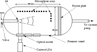
 , where
  the exit velocity and
  the exit
diameter; the Mach number is defined as
the exit
diameter; the Mach number is defined as  ; flow indicates the
presence of information on the flow field; acoustics indicates the presence
of information on the sound filed; the last column indicates the measurement
techniques for flow observation, with hot wires (HWA), laser-doppler
anemometry (LDA) and particle image velocimetry (PIV)
; flow indicates the
presence of information on the flow field; acoustics indicates the presence
of information on the sound filed; the last column indicates the measurement
techniques for flow observation, with hot wires (HWA), laser-doppler
anemometry (LDA) and particle image velocimetry (PIV)