


A sketch of the experimental setup was already shown in figure 4.
In a steel pressure/vacuum vessel a jet is released from a (cylindrical)
nozzle with a subsonic velocity. The ambient pressure in the vessel can be
varied between  and
and  bar. This allows us to vary the Reynolds
number of the flow without changing the Mach number or the physical
dimensions of the setup. The Reynolds and Mach numbers are defined as
bar. This allows us to vary the Reynolds
number of the flow without changing the Mach number or the physical
dimensions of the setup. The Reynolds and Mach numbers are defined as

 is only a function of the temperature and
can be kept approximately constant
is only a function of the temperature and
can be kept approximately constant  340 m/s for the temperature
equal to the ambient value. With a jet nozzle
340 m/s for the temperature
equal to the ambient value. With a jet nozzle  of say 10mm and an exit
velocity
of say 10mm and an exit
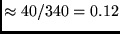
velocity  of 40 m/s the Reynolds number can in principle be varied
between, 400 and 400000 while the Mach number is constant
of 40 m/s the Reynolds number can in principle be varied
between, 400 and 400000 while the Mach number is constant
 . The lower value of Re can be easily calculated with help of
DNS and the higher value will be a challenge for LES. From
experiments listed in Table 1 it is known that
the dominant frequency of the sound
. The lower value of Re can be easily calculated with help of
DNS and the higher value will be a challenge for LES. From
experiments listed in Table 1 it is known that
the dominant frequency of the sound  is equal to

 is the Strouhal number (around 0.2-0.6 for a jet, depending on
the shape of the jet nozzle) , is again the jet exit velocity and
the jet diameter. With the numbers given above we expect a frequency of
is the Strouhal number (around 0.2-0.6 for a jet, depending on
the shape of the jet nozzle) , is again the jet exit velocity and
the jet diameter. With the numbers given above we expect a frequency of
 (note that this frequency is in principle
independent of the value of
(note that this frequency is in principle
independent of the value of  ). The acoustic pressure fluctuations and the
sound frequency
). The acoustic pressure fluctuations and the
sound frequency  (not equal to due to the Doppler shift) of the jet
are according to Goldstein (1974)
(not equal to due to the Doppler shift) of the jet
are according to Goldstein (1974)

 is the position of the observer,
  a non-dimensional constant,
 is the velocity fluctuation,
  the convective Mach
number, roughly half of the jet Mach number,
the convective Mach
number, roughly half of the jet Mach number,  the angle with the
main jet axis and the source frequency of the sound. Most microphones
measure
the angle with the
main jet axis and the source frequency of the sound. Most microphones
measure  while
while  is believed to be the quantity most closely related
to the sensation of loudness (see Goldstein 1974).
>From turbulence
theory we expect that
is believed to be the quantity most closely related
to the sensation of loudness (see Goldstein 1974).
>From turbulence
theory we expect that  scales with the jet velocity and
will more or less be independent of the Reynolds number. So in our
experiment we expect that the microphone output is mainly a function of and the angle
between the jet centerline and the observer.
To measure the acoustic field of the jet we will place (
scales with the jet velocity and
will more or less be independent of the Reynolds number. So in our
experiment we expect that the microphone output is mainly a function of and the angle
between the jet centerline and the observer.
To measure the acoustic field of the jet we will place ( )
acoustic pressure transducers (microphone) in the vessel. We will do this at
various different angles . Due to the small diameter of the jet
nozzle and the wave length of the acoustic wave (
)
acoustic pressure transducers (microphone) in the vessel. We will do this at
various different angles . Due to the small diameter of the jet
nozzle and the wave length of the acoustic wave (
 ) we need rather small microphones with physical dimensions
which are much smaller than
) we need rather small microphones with physical dimensions
which are much smaller than  . Such microphones are
commercially available.
. Such microphones are
commercially available.
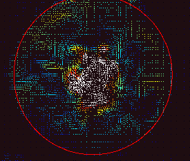
The acoustic field can be visualized with the Schlieren method.5 This method can be used to study the directivity pattern of the sound and acoustic reflection on the sides of the vessel. Detailed information about the structures in the flow, like vortices secondary motion, etc. can be obtained with Particle Image Velocimetry (PIV).6
 |
The statistics of the flow field can be obtained by PIV measurements or by Laser Doppler Anemometry (LDA) measurements.7Furthermore, we have to measure the temperature distribution in the vessel. We do not expect that at low velocities the temperature will play an important role but we also can not rule this effect out at forehand. For higher Mach numbers, which we want to study in a later stage, temperature effects will be important. The spatial temperature field can be measured with infrared thermography.
Another problem, put forward by Prof. M. Hirschberg of the TUE, will be the reflection of the acoustic waves on the wall off the low pressure vessel. To minimize this reflections we have to place acoustic damping material on the wall of the vessel. Such material is commercially available. If the damping of the acoustic reflections is not sufficient we have to incorporate the acoustic reflections in our simulation model.